Lab10
Introduction
In this lab, we implemented grid localization using Bayes filter. The robot is simulated following a preplanned trajectory and we determine where the robot is using Bayes filter at every iteration.
The structure Bayes filter is shown below:

In order to use Bayes filter to increase the accuracy, we need the following parts:
- State Space: The size in this lab is 12 x 9 x 18, 12 and 9 are the size of the plane, 18 is the size of angular space
- Belief: The belief of the robot at a given state
- Action Model: The probability that the robot arrive at state x’ from previous state x given input u
- Sensor Model: The probability that the robot has sensor reading z from state x
The prediction belief is calculated by prior belief and action model at the entire state space. Then it is corrected and normalized by the sensor model.
Code Implementation
Compute Control
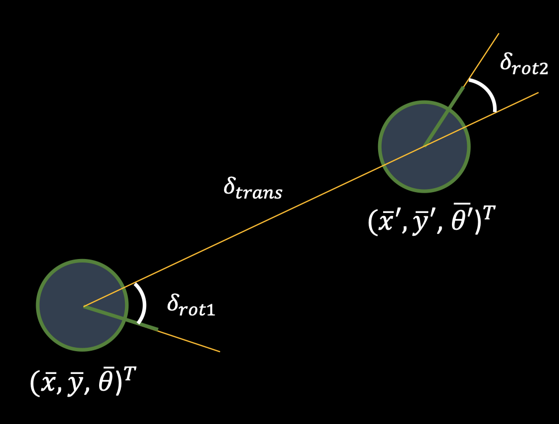
It calculates u based on a current and previous position. The principle is ilustrated in the graph below:

def compute_control(cur_pose, prev_pose):

    cur_x, cur_y, cur_yaw = cur_pose
    prev_x, prev_y, prev_yaw = prev_pose

    delta_x = cur_x - prev_x
    delta_y = cur_y - prev_y

    delta_rot_1 = np.degrees(np.arctan2(delta_y, delta_x)) - prev_yaw
    delta_trans = np.sqrt(delta_x**2 + delta_y**2 )
    delta_rot_2 = cur_yaw - prev_yaw - delta_rot_1

    return delta_rot_1, delta_trans, delta_rot_2
Odometry Motion Model
This describes the likelihood of achieving a current position given a control input and a previous position. u represents the actual control input calculated from odometry sensor reading. curr_pose and prev_pose are utilized to calculate u_compute for proposed control input.
We model the probability of the kinematic model of the Gaussian distribution.
- mu: mean value
- sigma: degree of dispersion
- x: the value that the probability is calculated
def odom_motion_model(cur_pose, prev_pose, u):

    u_compute = compute_control(cur_pose, prev_pose)

    rot1_val = mapper.normalize_angle(u_compute[0])
    trans1_val = u_compute[1]
    rot2_val = mapper.normalize_angle(u_compute[2])

    rot1_mu = mapper.normalize_angle(u[0])
    trans1_mu = u[1]
    rot2_mu = mapper.normalize_angle(u[2])

    prob_rot1   = loc.gaussian(rot1_val, rot1_mu, loc.odom_rot_sigma)
    prob_trans1 = loc.gaussian(trans1_val, trans1_mu, loc.odom_trans_sigma)
    prob_rot2   = loc.gaussian(rot2_val, rot2_mu, loc.odom_rot_sigma)

    return prob_rot1 * prob_trans1 * prob_rot2
Prediction Step
The prediction step requires two inputs: cur_odom and prev_odom, which represent the current and previous positions of the robot as detected by sensors. These positions are used to compute the control input u.
We have two groups of 3 layers loop in this function. The outside 3 layers loop traverse all the previous states. The inside 3 layers loop traverse all the current states. The transition probability is calculated by the previous state and current state.
Every prediction belief is the summation of all prior belief times transition probability. In order to accelerate the process, we only calculate the states that loc.bel (prior belief) is not zero.
Finally we normalize loc.bel_bar to make sure that the probability distribution add up to one.
def prediction_step(cur_odom, prev_odom):
    """ Prediction step of the Bayes Filter.
    """
    # get the control value given curr odom and prev odom
    u = compute_control( cur_odom, prev_odom )

    # init bel bar to all zeroes
    bel_bar_tmp = np.zeros((mapper.MAX_CELLS_X, mapper.MAX_CELLS_Y, mapper.MAX_CELLS_A))

    threshold = 0.0001

    for prev_x in range(mapper.MAX_CELLS_X):
        for prev_y in range(mapper.MAX_CELLS_Y):
            for prev_yaw in range(mapper.MAX_CELLS_A):

                if (loc.bel[prev_x, prev_y, prev_yaw] < threshold):
                    continue

                for cur_x in range(mapper.MAX_CELLS_X):
                    for cur_y in range(mapper.MAX_CELLS_Y):
                        for cur_yaw in range(mapper.MAX_CELLS_A):
                            cur_pose = mapper.from_map(cur_x, cur_y, cur_yaw)
                            prev_pose = mapper.from_map(prev_x, prev_y, prev_yaw)
                            transition_prob = odom_motion_model(cur_pose, prev_pose, u)

                            bel_prior = loc.bel[prev_x, prev_y, prev_yaw]
                            bel_bar_tmp[cur_x, cur_y, cur_yaw] += transition_prob * bel_prior

    # normalize to 1
    loc.bel_bar = np.true_divide(bel_bar_tmp, np.sum(bel_bar_tmp))
Sensor Model
The sensor model computes the probability that the sensor reading is correct given a state. It requires to return a 1D array of size 18 which is the likelihoods of each individual sensor measurement.
Like the motion model, we also model the sensor model as gaussian distribution. The input of gaussian function is the current sensor measurements that we took every 20 degrees during the turing around, which are stored in loc.obs_range_data.
def sensor_model(obs):
    """ This is the equivalent of p(z|x).
    """

    prob_array = []
    for i in range(mapper.OBS_PER_CELL):
        prob_array.append(loc.gaussian(loc.obs_range_data[i], obs[i], loc.sensor_sigma))
    return prob_array
Update Step
We dpdate the probabilities in loc.bel based on loc.bel_bar and the sensor model. It combines all the above functions.
we iterate through all the possible current poses of the robot by 3 layers of loops. For every possible pose, we find the prediction belief and multiply that by the measurement probability. Then we get the post probability.
Finally, we need to normalize loc.bel to make sure all its elements add up to one.
def update_step():
    """ Update step of the Bayes Filter.
    """
    for cur_x in range(mapper.MAX_CELLS_X):
        for cur_y in range(mapper.MAX_CELLS_Y):
            for cur_yaw in range(mapper.MAX_CELLS_A):
                bel_bar = loc.bel_bar[cur_x, cur_y, cur_yaw]
                obs = mapper.get_views(cur_x, cur_y, cur_yaw)

                measure_probs = sensor_model(obs)
                measure_prob_mul = np.prod(measure_probs)

                loc.bel[cur_x, cur_y, cur_yaw] = measure_prob_mul * bel_bar

    # normalize to 1
    loc.bel = np.true_divide(loc.bel, np.sum(loc.bel))
Demonstration
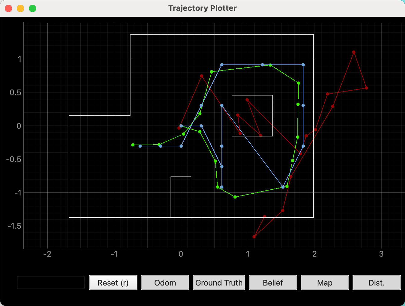
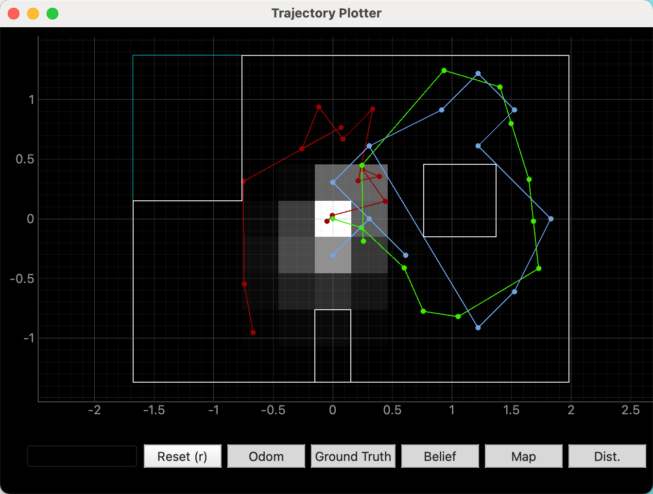
Green trajectory is ground truth; red trajectory is sensor reading; blue trajectory is calculated by Bayes filter.

We can also see the distribution of probabilities that different grids have.

This video demonstrate the whole process of how bayes filter works.