Lab7

1. Estimate drag and momentum

Choose your step responce, u(t), to be of similar size to the PWM value you used in Lab 6 (to keep the dynamics similar). Pick something between 50%-100% of the maximum u.

I choose 80% of the maximum u, so the pwm value is 210 out of 255.

The step response of the car is shown in the following graph:

fig, ax1 = plt.subplots()

color = 'tab:red'
ax1.set_xlabel('Time (s)')
ax1.set_ylabel('Distance', color=color)
ax1.plot(timestamps_s, distances, color=color)
ax1.tick_params(axis='y', labelcolor=color)

ax2 = ax1.twinx()  
color = 'tab:blue'
ax2.set_ylabel('Left PWM', color=color)  
ax2.plot(timestamps_s, left_pwms, color=color)
ax2.tick_params(axis='y', labelcolor=color)

plt.title('Distance and PWM vs. Time')
plt.show()

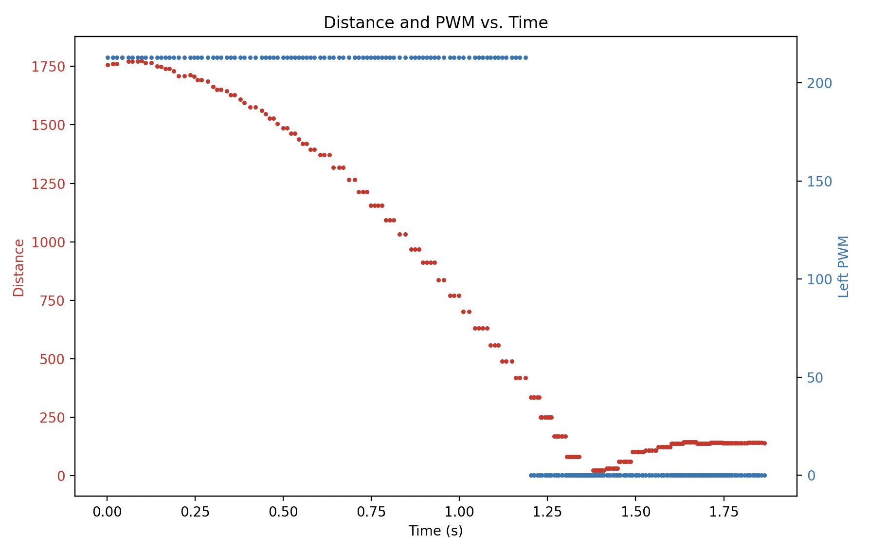
Because the distance sensor is operated in a non-blocking way, there are significant steps in the distance measurements. It brings errors in the velocity calculation. To solve this problem, I use interpolatation tool in numpy to guess the distance data between new sensor reading values.

# find non accurate data points
to_delete_idxs = []
for idx in range(1, length):
    curr_dist = distances[idx]
    if curr_dist == prev_dist:
        to_delete_idxs.append(idx)
    else:
        prev_dist = curr_dist
        
# interpolation
interpolated_distances = np.interp(timestamps_ms, new_timestamps, new_distances)

The new graph is shown as follows:

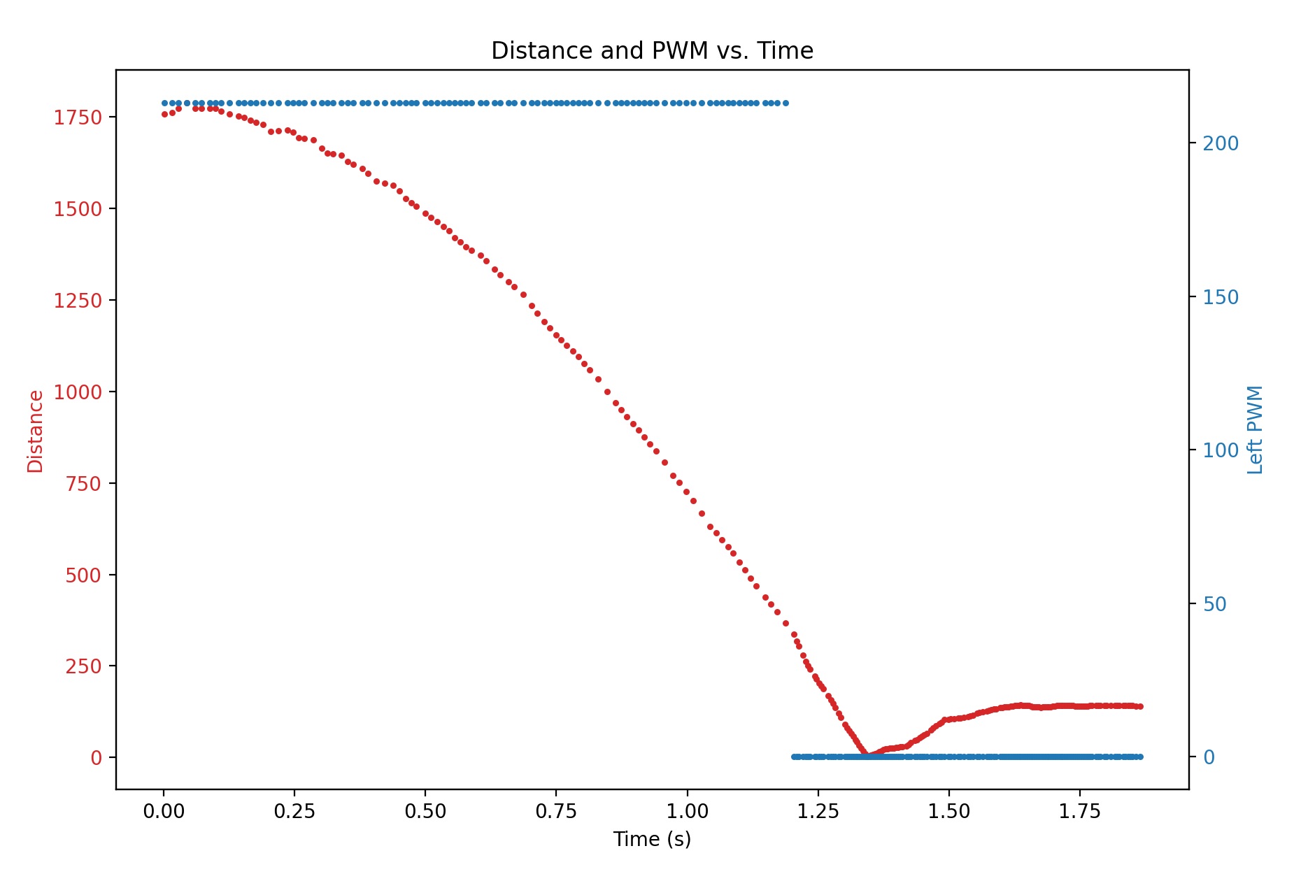
Make sure your step time is long enough to reach steady state (you likely have to use active breaking of the car to avoid crashing into the wall). Make sure to use a peice of foam to avoid hitting to wall and damaging your car.

The graph above indicates that the speed of car has reached steady state after 1.0s.

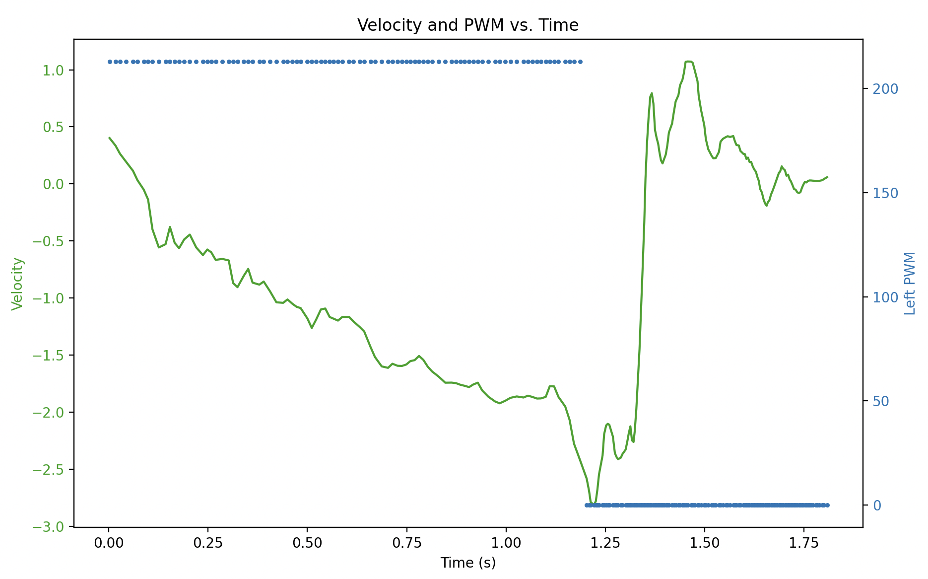
Show graphs for the TOF sensor output, the (computed) speed, and the motor input. Please ensure that the x-axis is in seconds.

I compute the speed based on interpolated distance data points, and use multupolynominal smoothing to make the curve of speed easier to analyze:

# calculate velocity based on distance
for i in range(1, length):
    velocities.append((distances[i] - distances[i - 1]) / (timestamps_ms[i] - timestamps_ms[i - 1]))
    
# polynominal smoothing
smooth_velocities = savgol_filter(velocities, window_length=16, polyorder=3)

The graph looks like this:

Measure the steady state speed, 90% rise time, and the speed at 90% risetime. (Note, this doesn’t have to be 90% rise time. You could also use somewhere between 60-90%, but the speed and time must correspond to get an accurate estimate for m.

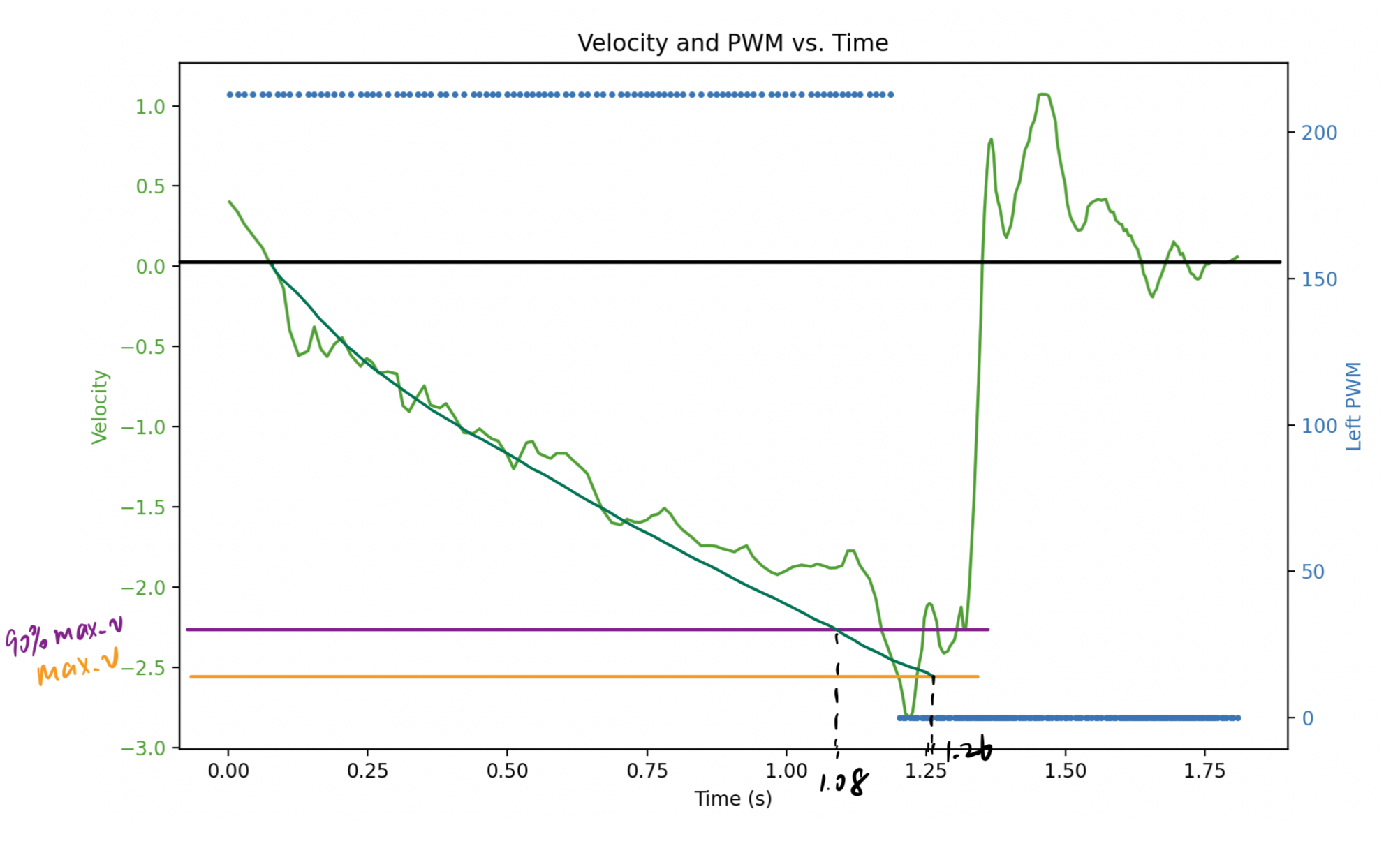
steady state speed: 2.5 m/s = 2.5 mm/ms

90% rise time: 1.08 s = 1080 ms

When sending this data back to your laptop, make sure to save the data in a file so that you can use it even after your Jupyter kernal restarts. Consider writing the data to a CSV file, pickle file

The data is saved to the output.csv file using the following code,

import pandas as pd
# Create a DataFrame
data = {
    'timestamp_ms': timestamps_ms,
    'distance': distances,
    'left_pwm': left_pwms,
    'right_pwm': right_pwms
}
df = pd.DataFrame(data)
# Save the DataFrame to a CSV file
df.to_csv('output.csv', index=False)

which looks like this,

# output.csv
timestamp_ms,distance,left_pwm,right_pwm
2,1757,213,147
17,1761,213,147
28,1761,213,147
44,1788,213,147
61,1772,213,147
72,1772,213,147
88,1772,213,147
......

Video of the car running at full speed toward wall:

2. Initialize KF (Python)

Compute the A and B matrix given the terms you found above, and discretize your matrices. Be sure to note the sampling time in your write-up.

\[d = \frac{u}{\dot{x}} = \frac{1}{2.5 \space mm/ms} = 0.4\] \[m = \frac{-d \times t_{0.9}}{\ln(1-0.9)} = \frac{-0.4 \times 1080}{-2.3} = 187.8\]

Now we have the estimation of parameter $d$ and $m$, we can calculate the matrix $A$ abd $B$。

\[A = \begin{bmatrix} 0 & 1 \\ 0 & -\frac{d}{m} \end{bmatrix} = \begin{bmatrix} 0 & 1 \\ 0 & -0.00213 \\ \end{bmatrix}\] \[B = \begin{bmatrix} 0 \\ \frac{1}{m} \\ \end{bmatrix} = \begin{bmatrix} 0 \\ \frac{1}{187.8} \\ \end{bmatrix} = \begin{bmatrix} 0 \\ 0.0053 \\ \end{bmatrix}\]

Using the following code, I find the average sampling time interval is 8.10 ms,

interval_sum = 0
for i in range(1, length):
    interval_sum += timestamps_ms[i] - timestamps_ms[i - 1]
interval = interval_sum / (length - 1)

So $\Delta t$ is set to 8.1ms

Descretize the matrices: \(Ad = I + \Delta t \times A \\ Bd = \Delta t \times B\)

Identify your C matrix. Recall that C is a m x n matrix, where n are the dimensions in your state space, and m are the number of states you actually measure.

\[C = \begin{bmatrix} -1 & 0 \end{bmatrix}\]

Initialize your state vector

x = np.array([[-distance[0]],[0]])

For the Kalman Filter to work well, you will need to specify your process noise and sensor noise covariance matrices.

\[\Sigma_u = \begin{bmatrix} \sigma_1^2 & 0 \\ 0 & \sigma_2^2 \\ \end{bmatrix}\]

Position stddev after 1s: $\sqrt{10^2 · \frac{1}{0.008}} = 111.8 \space mm$

Speed stddev after 1s: $\sqrt{10^2 · \frac{1}{0.008}} = 111.8 \space mm/s$ \(\sigma_3^2 = (20 mm)^2\)

3. Implement and test your Kalman Filter in Jupyter (Python)

Parameter settings are as follows:

d = 0.4
m = 187.8

A = np.array([[0, 1], [0, -d/m]])
B = np.array([[0], [1/m]])
C = np.array([[-1, 0]])

sig1 = 100
sig2 = 100
sig3 = 20

Sig_u = np.array([[sig1**2, 0], [0, sig2**2]])
Sig_z = np.array([[sig3**2]])

delta_t = 8.1

Ad = np.eye(2) + delta_t * A
Bd = delta_t * B

Kalman Filter process:

def kf(mu, sigma, u, y):
    
    mu_p = Ad.dot(mu) + Bd.dot(u) 
    sigma_p = Ad.dot(sigma.dot(Ad.transpose())) + Sig_u
    
    sigma_m = C.dot(sigma_p.dot(C.transpose())) + Sig_z
    kkf_gain = sigma_p.dot(C.transpose().dot(np.linalg.inv(sigma_m)))

    y_m = y - C.dot(mu_p)
    mu = mu_p + kkf_gain.dot(y_m)    
    sigma = (np.eye(2) - kkf_gain.dot(C)).dot(sigma_p)

    return mu, sigma

# init position state
x = np.array([[-distances[0]],[0]])
# init guess of uncertainty
sig = np.array([[5**2,0],[0,5**2]])

kf_state = []
for u, d in zip(left_pwms, distances):
    x, sig = kf(x, sig, [[u / 210]], [[-d]])
    kf_state.append(x[0])

Raw sensor reading value and kalman filter estimation:

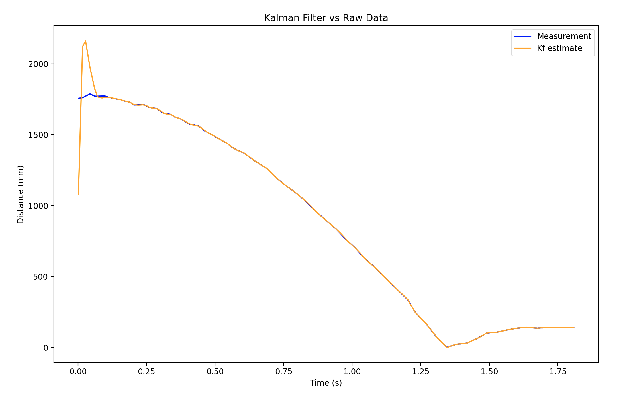
The larger sig_1 and sig_2 are, the less we trust the robot model, the larger sig_3 is, the less we trust the sensor reading. By adjusting the deviation value, we can find an appropriate way to combine the information of both snesor reading and model processing.

The prediction matches the sensor reading better as the standard deviation that I calculated for the robot model is large.